
Neural Networks can learn anything
A simple explanation on the basis of neural network learning
This is a question I’ve been recently asked, and I think it’s interesting enough to share about. A few people asked me how is it that machines can learn, and specifically, how is it that neural networks can learn to understand data that may be really complex. The goal of this article is not to give an in-depth explanation, but rather one that can be easily understood.
Everything is a function
We can think of functions in terms of an input and an output. The input is processed somehow and the output is defined solely by the input after passing on several steps that the function itself is.
That is a simple way of looking at them, and even without looking at the mathematical definitions, functions give you a relationship between the input and the output. The input is linked to the output through this function. The same input would always give you the same output.
Is it possible that a function does not give the same output by providing the same input? For instance, we might throw the same dice twice in the same way, and different numbers may come up.
Not really. There are variables that we’re not considering. Think about it this way: if we threw the same dice in the same way, where all the air atoms surrounding it had the same position and velocity, the gravitational pull from the Earth applied in the same way, with the dice bouncing in the table the same way and in the same spot… would we really get a different number? The answer is likely no: the concept stands, what we have just added are variables to the function. More inputs. This example might bring in the concept of randomness and feasibility for function approximation – but this is a subject for another day.
With this, everything that has some input and some deterministic output is defining a relationship between them, a level of correlation from these inputs to these outputs. That is our function.
Approximating functions
When we have a function we can give it several inputs and watch the outputs of each of them, we can even build a table that shows all the results for all our inputs. But if we don’t have the function, and instead we have a lot of inputs and their outputs… can we guess what the function was?
Yes, yes we can. This is, given that our dataset has certain attributes. Depending on the function, the exact way in which the function is defined may never be clear to us, but we can still approximate in a way that’s good enough for us to work. And this is an important concept: our approximation doesn’t have to be perfect, it only has to be useful enough.
In a real world example: we know that a lot of aspects make up for a particular house price, like the size of the lot, how old the construction is, and where it is located. And when we run calculations in our head, we round out prices to the thousands. The function we are approximating in our heads is not an exact match with the real-life function, but is still precise enough that we can make use of it. So, if in our head we came up with a price of $750.000, while the real life value was $750.823… we did an amazing job in estimating that house’s value!
A well approximated function can still be useful, even if it’s not the original, exact to-the-point function. Depending on the case, the amount of error that can be tolerated is different.
Linear approximations
The simplest way to approximate a function is to think of it as a linear combination of the variables it takes on. This means that we can multiply each variable’s input value to a factor (called weight) and sum up the results. This makes sense when you think about it: if a variable has no relation to the output at all, we can just multiply it by zero. If it has double the importance than other variables, then we multiply it by two. If the variable is inversely correlated with the result, then we multiply it by a weight lower than 1. And the same logic goes on for all of the variables.
It is tempting to think that with this, any combination possible is reachable, so we could come up with a good approximation to any function. However, this approach only works for functions that have a linear vector space. This means, functions where the possible results can be approximated by a linear combination of the inputs (what we just did). If this wasn’t the case, then choosing certain weights would work well for some inputs and would be awful for some others. This means that we haven’t really approximated the function, but rather a subset of the function’s domain. And this is not really useful.
Going over this again: a linear combination will only be able to approximate linear functions. But most of the real life functions are not linear. How do we approximate other ones?
Polynomial approximators
Well, we could extend our linear combinations to polynomic combinations. So a quadratic function can be approximated by a polynomial of grade 2 (i.e. a.x2 + bx + c). We can do the same for polynomials of grade 3, and 4, etc. In fact, we can keep doing this indefinitely, and Taylor series approximations is the mathematical demonstration that we can approximate any function with this.
But it may get tricky… we might end up with a really complex expression for a very simple function. For example, here’s a polynomial expression of grade 2 with 2 variables:
a.x2.y2 + b.x2.y + c.x2 + d.x.y2 + e.x.y + f.x + g.y + h
All letters except x and y are coefficients, the weights that we would need to adjust to get a good approximation. There’s 8 of them! And only with 2 variables and grade 2, which is not a powerful approximation at all. Just so you know, the same polynomial of grade 3 with 3 variables has 64 coefficients.
Global function approximators
Mathematically speaking, what we need to do for our function approximation to be able to learn any function is to introduce a non-linearity. Polynomials are a way, but not the only way. Non-linearities will break the monotony of the linear approach we have taken so far. They will allow the vector space that we can reach to be the full space of functions possibly defined with these variables. This means that no matter what strange function we’re trying to approximate, we’ll be able to adjust our weights in a way that we can have a good prediction for outputs.
These non-linearities, in neural networks are called activation functions. There are a bunch of activation functions, but one of the most popular today can be even done in our head: Leaky ReLU (stands for Leaky Rectified Linear Unit – a story for another day). It goes like this: if the variable is lower than zero, we multiply it with a small value (like 0.1). If the variable is higher than zero, we leave it as it is.

This is enough that our approximation to our function can be achieved.
Neural Network Architecture
All that only guarantees that our approximator (neural network) can achieve a good approximation of the function in theory, but a few conditions need to occur. For instance, we need to consider all inputs, and we need to consider the complexity of the correlations. Since we are approximating, we don’t know what that complexity is, but we can have an idea based on the domain. This means that how variables may be correlated to make a medical condition diagnosis may require more complexity than, let’s say, calculate how much gas a car will spend in a trip.
And we won’t know for sure until we learn this correlations – so how can we do something that works regardless?
At this point, the architecture of a neural network is what makes this work. Architecture meaning the way in which we will work with this data until we reach a prediction. Architectures setup the way for us to stack learnt correlations into a complex network of deductions.
Nodes
Think of every “node” of the network as our first linear combination approach, together with the activation function on that linear result. Every node will be different in that it will use different weights for each variable. If we have two nodes, it means we can “learn” that sometimes a variable is very important and sometimes it is not.
Each node will learn some kind of correlation between an input, and an output, in the same way that we want to do with our global result. It means that solving a big function will be just the combination of solving different small functions. Learning a small function is simpler than a big function, and then we just need to learn how they correlate.
Let me give you a few examples of how different weights can relate to different functions.
- One input x and one node with one weight w. If we have w = 2, then we just learned the function “double”! Our approximation of the function will be activation(w.x) = 2x for every positive x.
- Two inputs, x1, x2 and that our weights w1, w2 are set to 0.5 each. This is the average function! Our approximation will be activation(x1.w1 + x2.w2) = 0.5x1 + 0.5x2 = (x1 + x2) / 2.
Each node will be a function of its own. And as we’ve seen so far, they’re limited, but power comes in numbers.
Stacking nodes
By stacking more and more of these “little functions” we can create more complex functions. The functions can get as complex as needed to reach a good prediction value.
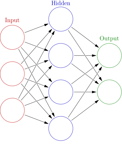
In network architecture, we say that the network will have input nodes, that operate directly on our input values, hidden nodes, that operate on values that are not inputs to the network, but rather created by the network itself, and output nodes, for which the result will be used as the prediction of the entire network.
Actual learning
So it all comes down to finding the right weights. How does a network do that?
In the very simplest way you can imagine: it takes a guess. It compares the result with the real output (remember our dataset?). And it adjusts weights so that the next time it gets a little closer. Iterating lots of times will actually give a good approximation!
The process of guessing is called forward-propagation, because the values move “forward” from the input to the final nodes of the network to give a prediction. The process that is applied to adjust the weights is called back-propagation, because it starts with the output and works its way through the network. Details on this for another day – there’s some math involved that I’d like to keep out of this first approximation to the subject.
Conclusion
That’s it! It’s all about multiplying and adding numbers so that we can reach a good prediction on the result. This will be done through some parameters we call weights, and having the right weights will mean that we have correctly approximated the function we wanted to learn.
This very basic explanation and over-simplification on how neural networks work is meant to get only one point across: any function can be approximated by them, given only these conditions:
- the input data is available,
- the output data is available to verify,
- the network has a sufficiently complex architecture to construct the correlations between data points (features),
- and the activation functions had been correctly chosen to identify non-linearities.
Secondary take away
Today I hopefully introduced the following concepts in a reachable manner:
- functions
- linear combination
- non-linear combinations
- inputs
- outputs
- weights
- data correlation
- function vector space
- activation function
- neural network nodes
- neural network architectures
I would like to expand on several of these topics, AI related, always trying to make them graspable. Please, reach out to me with what would be the concept that you’d like me to tackle next, or which one discussed here is not yet clear enough – I need to learn to explain them too! (Or at least, approximate to it!)